
Gravity Spy Machine Learning by Machine Learning
Machine learning offers powerful tools for performing complex tasks – its applications are broad in scope, and virtually limitless given sufficient resources. Within Gravity Spy, armed with the ever-growing dataset of detector glitches classified by our volunteers, we are able to construct an algorithm that can not only identify glitches in detector data, but distinguish between different glitch types with impressive accuracy. ChatGPT is another application of machine learning that has been hitting the headlines recently. It is notable in being able to write detailed text in response to prompts. To illustrate its potential, I asked to summarise the inner workings of the Gravity Spy machine learning classifier. Its response is below, unedited (except for some visual aids I have provided)…
At the heart of the Gravity Spy project is a machine learning algorithm called a convolutional neural network (CNN). CNNs are a type of deep learning algorithm that are particularly effective at image recognition tasks. CNNs are particularly well-suited to analysing complex data such as the spectrograms produced by gravitational wave detectors. These spectrograms represent the frequency and intensity of the detector output over time, and can be thought of as a two-dimensional image.
The Gravity Spy CNN consists of multiple layers, each designed to extract increasingly complex features from these input spectrograms. The first layers are convolutional layers, which apply a set of learned filters to the input image. These filters are designed to highlight specific features in the image, such as lines, edges, or curves. The convolution operation involves sliding the filters over the input data, multiplying the values at each location, and summing the results.

The output of the convolutional layers is passed through max-pooling layers, which downsample the output by selecting the maximum value in each neighbourhood. This reduces the dimensionality of the output, making the model more efficient while preserving the most important features. This process is repeated with multiple filters to generate a set of feature maps for each layer of the network. Finally, the output from the last convolutional and pooling layers is flattened and fed into one or more fully connected layers, which produce the output glitch classification. These layers use weights to connect every neuron in one layer to every neuron in the next layer, allowing the network to learn complex relationships between the extracted features and the corresponding glitch that they were derived from.

To train the Gravity Spy CNN, a large dataset of labelled examples is required. Citizen scientists contribute to this effort by classifying glitches on Zooniverse. The CNN is trained using an optimization algorithm to minimize a loss function, with the cross-entropy loss function being used in the case of Gravity Spy. Cross-entropy is a measure of the difference between the predicted probabilities and the true labels for each example in the training set. By minimizing the cross-entropy loss, the CNN is able to learn to make increasingly accurate predictions about which glitch class each spectrogram belongs to. This minimisation is achieved by finely tuning the parameters of each layer of the CNN in an iterative fashion.
One of the key contributions of the Gravity Spy project has been the identification of new classes of glitch. These include the Crown (also known as Fast Scattering), Pizzicato, Paired Doves, and Helix classes. Paired Dove and Helix classes were identified during early beta testing of Gravity Spy on Zooniverse, while Crown was particularly common during the third observing run of LIGO. Pizzicato, which looks like a UFO in spectrograms, was recently identified, and is thought to be related to violin modes in the LIGO detector’s suspension system. The Gravity Spy CNN can easily incorporate these new glitch classes, and by properly sub-dividing existing glitch classes into new ones their origins in the detectors can be better identified.
In conclusion, the Gravity Spy project is an excellent example of the power of citizen science and machine learning in advancing our understanding of the universe. By harnessing the collective intelligence of volunteers on Zooniverse and using a CNN trained on a large dataset of labelled examples, the project has made it possible to distinguish true gravitational wave signals from noise and identify new classes of glitch. As machine learning technology continues to improve, we can expect to see similar projects emerging in other areas of science, enabling us to tackle ever more complex and challenging questions.
Impressive (and perhaps a little unnerving)! ChatGPT knew a lot about Gravity Spy and convolutional neural networks by default. It did need to be told about the new glitch classes, and the specifics of the layers used in our network, but once told, it was able to write about them, as you can see! I didn’t tell it to say that Gravity Spy is excellent.
The key to ChatGPT’s remarkable abilities is the vast high-quality training dataset provided to it. Without this dataset, it would not be possible to produce such powerful generative algorithms. In a similar vein, the Gravity Spy classifier’s incredible capability to classify glitches in gravitational wave detector data is only possible because of the high-quality dataset of labelled glitch classifications it is provided: the work of our volunteers!
- Christian Chapman-Bird, on behalf of the Gravity Spy team.
Research Spotlight: Recent Gravitational-Wave Glitch Studies
We’re learning more about glitches in gravitational wave detectors all the time. The most recent LIGO–Virgo–KAGRA Collaboration meeting (12–16 September 2022) in Cardiff featured the latest progress on our detectors and data analysis. Many research projects were presented as posters: several were looking at topics related to glitches, and many used results from the Gravity Spy project for some part of their work! We’ve reached out to authors of these posters to spotlight their work in this blog post. Below you’ll find brief summaries about these research projects, and a glimpse into some of the science that contributing to Gravity Spy can enable.
Investigations of Increased Detector Noise due to Trains at LIGO Livingston – Jane Glanzer (LSU)
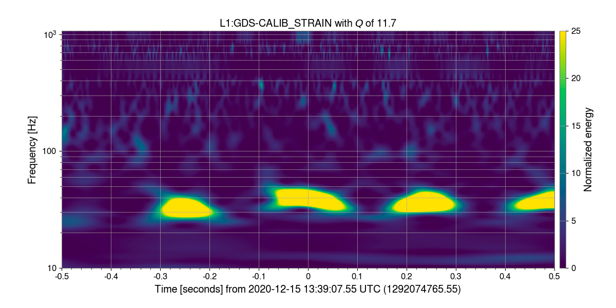
Scattered light is one of several types of noise sources present in the LIGO detectors. Specifically, Fast Scattering (known as Crown in Gravity Spy) is a type of scattering that occurs with increased ground motion in the 1-6 Hz (anthropogenic) and 0.1–0.3 Hz (microseism) band. Its structure takes the form of small arches present in time frequency space.
Scattering happens when light from the main laser path is scattered by a mirror reflected by another surface. A fraction of this scattered light can rejoin the main path, and introduce noise back into the main gravitational wave data channel. Environmental seismic disturbances contribute to the production of scattered light and limited detector sensitivity.
Trains near the LIGO Livingston detector are one of the main causes for increased seismic motion. Through the use of the linear regression tool LASSO, we searched for narrow band seismic frequencies to determine possible detector couplings responsible for these fast scattering glitches. This is done by looking for correlations between increases in ground motion and the calibrated strain data. The results find that the most common seismic frequencies that correlate with increases in detector noise are 0.6–0.8 Hz, 1.7–1.9 Hz, 1.8–2.0 Hz, and 2.3–2.5 Hz. In the Livingston detector, the arm cavity baffles and cryobaffles have resonances such that they may be the culprits for some of the Fast Scattering seen in O3 due to the train motion.
ArchEnemy: Subtracting scattered light artefacts from gravitational-wave data – Arthur Tolley (Portsmouth)
While the LVK have observed ~90 gravitational-wave signals to date, searching for these signals in the gravitational-wave strain data isn’t easy! This is made more complicated by the presence of random bursts of noise, known as glitches, in the data.
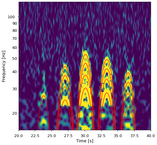
A very common glitch seen in the third observing run is caused by the scattering of light within the gravitational-wave detectors, colloquially called Scattered Light. I have been developing the ArchEnemy pipeline which can find these glitches and remove them from gravitational-wave data. We model scattered light glitches and produce a template bank of scattered light templates to matched filter with gravitational-wave data, allowing us to identify these glitches in a manner similar to how we search for gravitational-wave signals. Following the identification of the best fitting template for each scattered light glitch in the data, we can clean the gravitational-wave data by subtracting them. Cleaning gravitational-wave data can uncover previously obscured gravitational-wave events and will ultimately improve the sensitivity of the detectors.
A random forest classifier to distinguish between chirps and glitches – Neev Shah (UBC)
Glitches can often hinder the search for gravitational waves by showing up as false candidates. We develop a new statistical distinguisher that can distinguish between different types of glitches and chirps. Assuming all events as real signals (glitches are not!), we project them onto a gravitational-wave model to infer the (posterior) probability distributions of their astrophysical parameters. We extract particular features from these posterior distributions and use a tool called Random Forests for the purpose of classification. Random forests can identify spatial clusterings in the parameter space that can help separate different classes of glitches and gravitational waves.
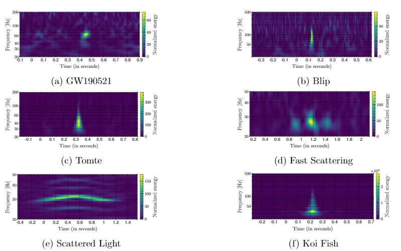
We find that for specific astrophysical parameters like the mass and spins of the binaries, the posteriors for glitches are starkly different from those of simulated gravitational waves, and the random forest can identify them to separate different glitch families and gravitational waves. We train our model using hundreds of simulated gravitational waves and thousands of glitches from 5 glitch families (Blips, Tomtes, Koi Fish, Fast Scattering and Scattered Light) that were pre-classified by Gravity Spy! We find that our method can be quite useful for the purpose of classification as it has an overall accuracy of about 97% and a Chirp recall of about 90%. This tool might help in future observing runs when there would be a lot of candidate events, and a large number of glitches among them.
GSpyNetTree: Improving Gravity Spy classifications toward O4 – Sofía Álvarez-López (UBC)
When detecting gravitational waves, removing glitches is one of our most significant challenges. Gravity Spy has helped us classify many of these glitches, proving very helpful for LIGO detector characterization. However, as one of LIGO’s core missions is the detection of gravitational waves, it is worth focusing on their search. In this sense, we discovered that Gravity Spy has the potential to be more than a glitch classifier: a gravitational wave vs glitch classifier!
Nevertheless, we had to restructure Gravity Spy to do so. Moreover, in the context of the 4th LIGO–Virgo–KAGRA observing run, new challenges arise in gravitational-wave classification, as detectors are expected to be more sensitive. The possible appearance of new glitches, and the likely occurrence of overlapping glitches and GWs (as shown in the image above), suggest the need for a new model for GW classification. We studied how Gravity Spy responded to these challenges and developed GSpyNetTree, the Gravity Spy Convolutional Neural Network Decision Tree: a gravitational wave vs glitch classifier that aims to tackle these challenges.
Towards unified modelling of astrophysical and background populations – Jack Heinzel (MIT)
One of the challenges of LIGO analysis is identifying which signals are astrophysical in origin and which signals are environmental noise. Recent progress has been made in identifying common signatures of Gravity Spy-identified environmental noise, which are unlikely to occur for real astrophysical gravitational waves.
In particular, when environmental noise is analyzed as a coalescence of a compact binary, the (nonphysical) parameters corresponding to the signal are so different from parameters we usually observe in astrophysical signals that we can confidently separate the noise population from the astrophysical population. We can then analyze the properties of events which are more ambiguous in origin, simultaneously estimating the probability of astrophysical vs terrestrial origin. The astrophysical information is then folded in to constrain the population of astrophysical events.
That’s all from us. Once again, a big thanks for all the classifying you’ve all done so far: as you can see, we’re chipping away at the glitch problem but there’s still plenty of work to be done!
- Christian Chapman-Bird, on behalf of the Gravity Spy team.
Introducing plans for Gravity Spy 2.0!
Hey GravitySpy-ers,
We are excited to announce that the Gravity Spy team was awarded a three-year research grant by the U.S. National Science Foundation (NSF) to build the next volunteer-enabled gravitational-wave search phase. The project will investigate approaches to use auxiliary channel data, the same data used by LIGO scientists when isolating other noise signals from the glitches in the main channel. Existing volunteer efforts engaging in advanced work (e.g., reading and interpreting information in alogs and providing insights into the root causes of glitches) typically performed by scientists at the detector sites inspired the research team to consider additional technical support to assist volunteers. A recent publication by the research team (Soni et al., 2021) demonstrated that volunteers are pretty good at making discoveries in large data sets even without such technical support.
The new project is complex, which is why we have built a team of researchers from across the U.S., including LIGO researchers within CIERA, LIGO researchers at Christopher Newport University, machine learning researchers at Northwestern University, and crowd-sourced science researchers at Syracuse University and the University of Wisconsin-Madison.
One goal of the project is to create novel interfaces for Gravity Spy that visualize the auxiliary channel data and provide statistical summaries about correlations between glitches, activities performed by LIGO scientists when they investigate the source of glitches. The team plans to create Beginner, Intermediate, and Advanced workflows that support different modes of interaction at each stage. In the Beginner mode (see Figure below for an interface mockup), volunteers will be able to compare a glitch that occurred in the gravitational-wave channel with the spectrogram of correlated auxiliary channels to assess whether the correlation seems natural or coincidental. In Intermediate mode, volunteers will be able to examine and refine collections created by beginners and identify correlations between glitches and the auxiliary channel over some timeframe. Finally, work in the Advanced mode will enable volunteers to discover the root cause of glitches by examining patterns and making inferences among large sets of auxiliary channel data.
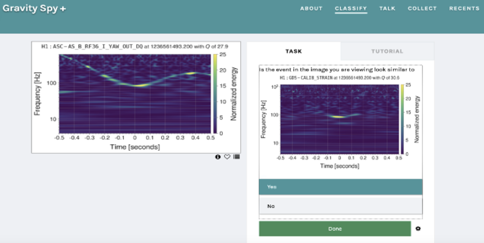
By building tools to support similar activities in Gravity Spy 2.0, volunteers will view new data and learn to make statistical inferences about noise signals among the thousands of auxiliary channels. Over the next year, the research team hopes to understand what background knowledge of the auxiliary data is helpful for volunteers, and what system tools and expertise will help volunteers identify connections among data sources. Through this, the research team hopes volunteers will isolate which relationships are causal vs. spurious. The research team will engage existing Gravity Spy volunteers throughout the project to obtain feedback and insights about the new interfaces (a mockup interface is shown below). We hope everyone is as excited about this project as we are.
We look forward to continued collaboration with volunteers as Gravity Spy sets the standard for the next generation of people-powered science projects.
Cheers,
The Gravity Spy Team
New Glitch Category Added to Gravity Spy – Pizzicato!
Hello everyone!
Pizzicato (originally known as High Frequency Burst 500 Hz) has been added as a new glitch category option in Level 5 and Level 7!

Pizzicato was brought to our attention when it was proposed as a new glitch class by @EcceruElme. She, along with the help of other users, is ultimately the reason why Pizzicato has been added as a new category.
Pizzicato glitches typically resemble a UFO and show up within the frequency ranges of First Order (~500 Hz) and/or Second Order(~1000 Hz) Violin Modes. Pizzicato first showed up during Engineering Run 14 (ER14), and continued to the end of O3. About 80% of these glitches are found at the Livingston detector, with the other 20% occurring at Hanford. They showed up in both detectors within months of each other; however, since we have seen possible previous incarnations of Pizzicato (see Church), we cannot be certain that whatever is causing these glitches is something completely new to the detectors.
This glitch is so interesting to us primarily because it so clearly seems related to the violin modes of the test mass suspensions, but at the same time we haven’t yet been able to pinpoint an exact cause.
Violin modes occur when the glass fibers that hold up the test masses (the mirrors that we bounce lasers between to measure gravitational waves) in the detectors experience excitations from changes in temperature. These excitations manifest in the fibers at around 500 Hz and, depending on how strong these excitations are, can cause vibrations at higher frequencies, similar to how plucking a violin string can cause reverberations at multiple frequencies. Excitations around 500 Hz are First Order Violin Modes, 1000 Hz are Second Order, and 1500 Hz are Third Order Violin Modes.
Comparing Spectra
Since these glitches are present in the same frequency ranges that Violin Mode Harmonics glitches take place in, the first thing we checked was if Pizzicato glitches were directly correlated to the violin modes being excited. We did this by first finding a time where a Pizzicato glitch was seen, and then picking a nearby time where there were no nearby glitches (Fig. 1 below). We then plotted data from these times as a spectrum (Fig. 2 below), which shows us the Amplitude Spectral Density (ASD) versus frequency. The ASD shows us the average amount of noise in the detectors at any given time.

Note: BNS Range y-axis units not shown for viewing clarity.
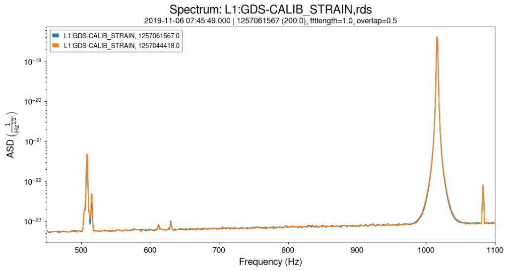
The blue in Figure 2 above gives us the ASD at the time of the glitch, and orange is a nearby time that didn’t contain any glitches in this frequency range. Both spectra line up perfectly, which tells us that the violin modes were present in this exact capacity during both times, but Pizzicato wasn’t. This tells us that Pizzicato could not have been caused by a change or gain in the amount of violin modes present in the detector. After comparing several Pizzicato glitch times to nearby times, it seemed like the biggest takeaway was that when the Pizzicato glitch was centered around 500 Hz, the spectra during the lock time showed the ASD as being higher around 500 Hz than 1000 Hz, and vice versa for glitches centered at 1000 Hz.
Comparing to Violin Mode Changes in Amplitude
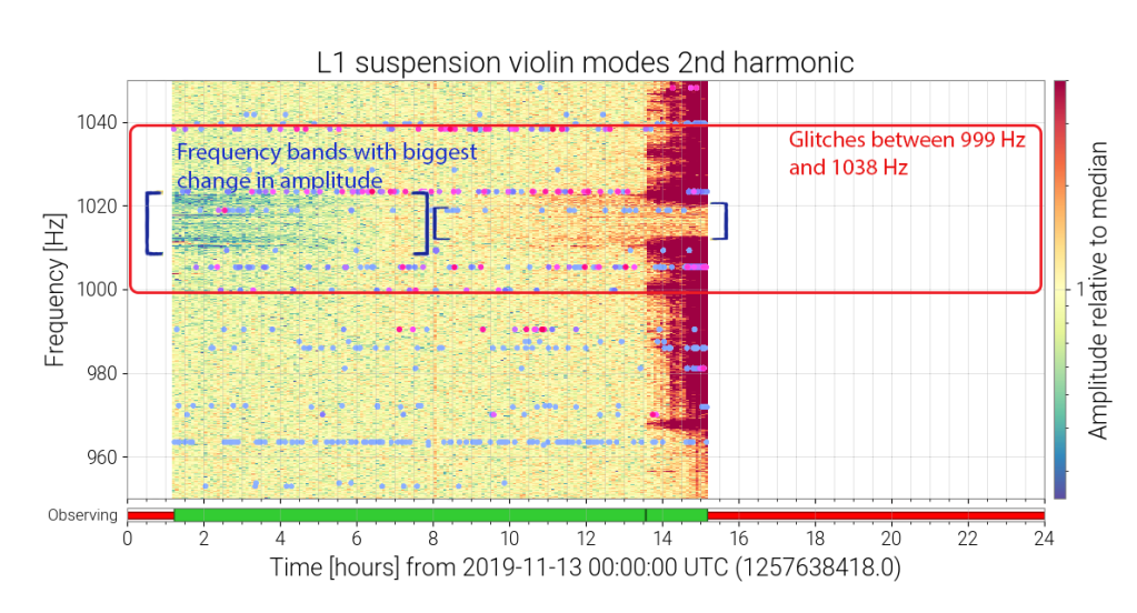
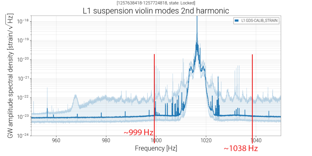
Below (Fig. 3) is a day where Pizzicato glitches were cropping up in the Second Violin Mode frequency range, between 999 Hz and 1038 Hz. There are multiple lines of glitches (dots) laid over the amplitude of the Second Order Violin Modes relative to the median amplitude. The confirmed Second Order Violin Mode frequencies that Pizzicato glitches occur at are 999 Hz, 1005 Hz, 1018 Hz, 1023 Hz, 1028 Hz, and 1038 Hz. We can see lines of glitches at all these frequencies. This tells us that the glitches in these lines are very likely Pizzicato.
You will also notice in Figure 3 that there seems to be a blue band between 1009 Hz and 1023 Hz and a red band between 1013 Hz to 1018 Hz where the amplitude of the violin modes seems to be heightened. We are not sure if that has anything to do with Pizzicato, but I thought I would note it anyway since we know that 1018 Hz and 1023 Hz are proven to be the peak frequencies of some Pizzicato glitches.
Looking at the spectrum in Figure 4 below that gives us the ASD of the Second Violin Modes for this date, we see that the range where these higher frequency Pizzicato glitches occur also happens to encompass the majority of the range where Second Order Violin Mode Harmonics are seen ringing up.
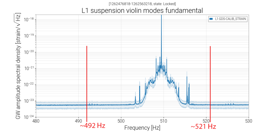
Below (Fig. 5) is another day where we were seeing Pizzicato, but this time the glitches are seen between 492 Hz and 521 Hz, which corresponds to the First Order Violin Mode frequency range. We determined that these lower frequency Pizzicato glitches can occur at 492 Hz, 496 Hz, 510 Hz, 514 Hz, and 521 Hz. Again, these frequencies line up with multiple lines of glitches on the glitchgram, although in this example we also see lines of unknown glitches at frequencies Pizzicato is not currently known to occur at.
Like the previous example, we also have a frequency band, between 505 Hz and 515 Hz, where the First Violin Mode amplitude is changing relative to its median, however, we do not see any similarities between the frequencies for the changes in amplitude here and the frequencies Pizzicato manifests at.
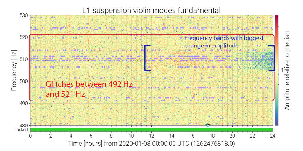
Figure 6 below, similar to Figure 4, shows a spectrum that tells us that the frequencies that these lower frequency Pizzicato glitches occur at spans the entirety of the frequency band for the First Order Violin Modes. Because of this, it’s hard to determine whether Pizzicato is or is not a direct outcome of the violin mode harmonics.
So then what causes Pizzicato? Why do they occur at these particular frequencies? The evidence doesn’t lead us in a particular direction, so we can only speculate for now.
A theory for what may be causing Pizzicato are the damping mechanisms for the violin modes. Since violin modes generate a lot of noise in the detector, LIGO has multiple ways to dampen the fibers, and it’s very possible that one of the many systems put in place to dampen them is causing a glitch to appear in the main channel. This theory is supported by the fact that Pizzicato glitches around 500 Hz seem to be correlated with lock stretches of higher First Order Violin Modes, and glitches around 1000 Hz appear when Second Order Violin Modes are particularly high.
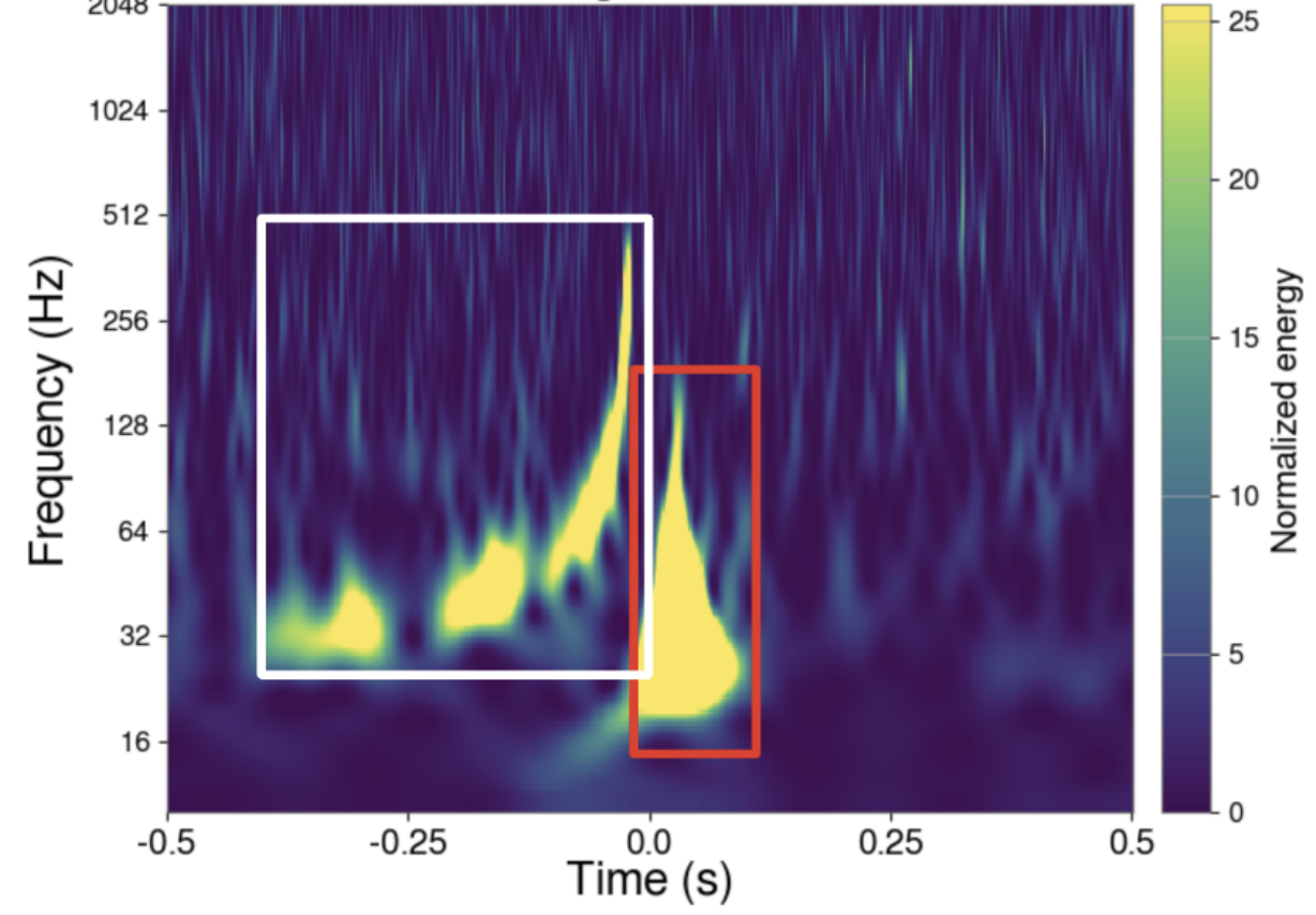
On the other hand, it is also possible that Pizzicato glitches are indeed directly caused by violin modes. If they are a direct result, it would be very interesting to compare them to the Violin Mode Harmonics glitches (Fig. 7) that we already keep track of in Gravity Spy, especially since they have similarities in frequency but are otherwise extremely different in terms of morphology, duration, variation over time, and in how they appear in the detectors – Violin Mode Harmonics like to string together whereas Pizzicato glitches don’t.


We will be continuing to explore possibilities and other avenues of looking through the data and hope we can update you all soon!
We want to thank everyone who interacts on Talk, proposes categories, and creates collections. It really helps the gravitational wave community! If you haven’t already, check out our recent announcement of the discovery of two separate Neutron Star – Black Hole Mergers! Discoveries like these would not be happening nearly as often without the dedication of citizen scientists like you!
Oli Patane and the Gravity Spy Team
New O3 Glitch Options
Hi all,
Backed by popular demand, we have added a few new classes of glitches that are prevalent in the O3 data. You will see these options available if you are classifying on the “Binary Black Hole Merger” or “Inflationary Gravitational Waves” workflows.
70 Hz Line:
These are strong, monochromatic lines that started appearing in O3 and sit at around 70 Hz.

Crown:
These are repeating, arching glitches at frequencies of ~20-50 Hz and appear in groups of ~3-5.

High Frequency Burst:
These are short-duration, blip-like glitches that occur at frequencies greater than ~1000 Hz.

Happy classifying!
Mike
Diagnosing the Tomte glitch
Hi everyone!
Recently, some of LIGO’s detchar experts investigated the connection between Tomte glitches from Gravity Spy and the bias voltage on a particular circuit. You can read the full alog of this investigation here. Below is a summary written by TJ Massinger, one of the detchar experts who does a lot of work with Gravity Spy data!
During recent commissioning work at the LIGO Livingston Observatory, it was noticed that glitches were occurring while the bias voltage on a circuit (an electrostatic actuator) was adjusted. Inspection of these glitches using the same time-frequency visualization that Gravity Spy uses showed that they looked qualitatively similar to glitches classified by users as the “tomte” class.
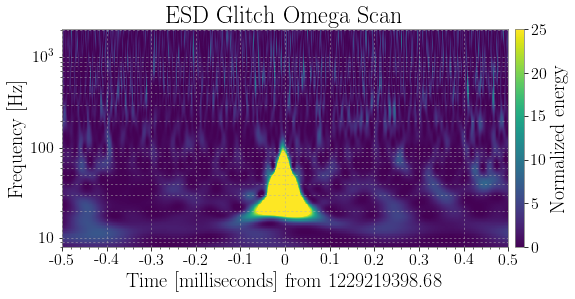
Spectrogram of an ESD bias ramping glitch.
Using the GravitySpy classifier, it was found that these recent glitches are also classified as tomte glitches. To quantify the similarity of the bias voltage glitches to the tomte glitches seen in the second observing run (O2), GravitySpy was used to gather a collection of previously identified tomte glitches in O2 with parameters similar to those seen when adjusting the bias voltage. Upon comparing these populations, their time- and frequency-domain morphology was found to be nearly identical, suggesting that the population of tomte glitches in O2 might be understood by continuing to investigate the glitches that occur when adjusting bias voltages.

Tomte rate in O2 based on Gravity Spy classifications with greater than 90% confidence.
Engineering Run 13
Hey GravitySpy-ers,
We are excited to bring you new data from our Engineering Run 13! Data taken during Engineering Runs are meant to test not only some of our new upgrades to the detectors but some of our software (like Gravity Spy).
When
Dates: 10 am Central Time Dec 14 to 8 am Central Time Dec 18 (N.B. Due to some issues at the sites science ready data was not available until Saturday December 15)
What Detectors Are Running
Originally, we anticipated only having Hanford and Virgo due to critical repairs at Livingston. These repairs, however, completed yesterday and after a short delay Livingston has joined ER13. At first, we will be streaming in the data live for Hanford and Livingston over the weekend, and at a later date will add Virgo ER13 data to the Virgo only workflow.
What’s New
The sensitivity of the LHO detector has increased its range to detect binary neutron stars from 80Mpc to 90Mpc, LLO has increased to 100Mpc and Virgo has nearly doubled its range from 25 to 43Mpc. A number of different glitch classes have arisen and the engineering run is a golden opportunity to identify and eliminate these so we can be rid of them for the year long O3 run which is anticipated to start in March 2019.
Example: https://alog.ligo-la.caltech.edu/aLOG/index.php?callRep=41765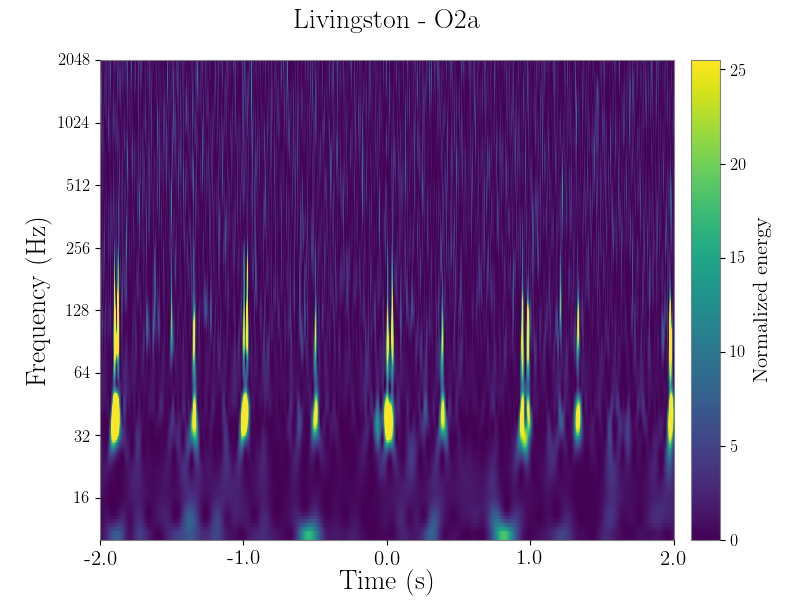
Some of the changes at both LHO and LLO that have led to this improvement include squeezed light and a new 70W laser amplifier that will improve LIGO’s quantum noise limit. In addition, Acoustic Mode Dampers will damp internal modes of the test masses to reduce parametric instability (light interacting with mirrors as positive feedback). Also, there was a change of several test masses to improve their coatings (especially for green light) and to remove a point absorber at LHO.
We look forward to your collections of interesting new glitches and for determining the cause of the new excess noise sources!
The Gravity Spy Team.
Introducing Virgo and a new workflow structure!

Hey Gravity Spiers,
We are really excited to finally introduce a new detector, workflow structure, and tool this week. First, we present a new workflow containing glitches from the Virgo detector in Pisa, Italy. Second, we are changing the level structure to speed up our user training. Finally, we are bringing you an auxiliary web tool to help the search for unique and novel glitches.
Virgo

Virgo differs from Hanford and Livingston in a few ways including the length of the arms, the apparatus holding up the test masses, and the suspensions. We anticipate there will be a number of interesting new glitches in Virgo. For some glitches, such as Scattered Light, they will appear different but have the same cause. For other glitches, such as the Violin Mode Harmonics, they will be the same source but at different frequencies due to the different suspension system. Below we demonstrate a few novel glitches you may find along the way while classifying Virgo glitches, including a new class we have called Fireball (bottom right).


New Workflow Structure

For those of you familiar with Gravity Spy’s training method, we intend to utilize pre-labelled images to help train new users in the classification task. In addition, in order to facilitate training, we introduce a different number of new families of glitches in different levels, culminating in Level 4 where all 22 classes are introduced. However, after some feedback, as well as looking at the data, we learned that getting from level 4 to level 5 was taking longer than anticipated. We decided that this was due to too many new classes being introduced between level 3 and 4. Specifically, the amount of pre-labelled images users were seeing was spread out across too many new classes causing the number of classifications a user must complete before seeing pre-labelled data to sky rocket. Therefore, we are adding another intermediate level that has 15 classes. We believe this will cause users to see pre-labelled images of the new classes faster and, in turn, move through the levels faster. In total, with the addition of Virgo, there are now 7 levels in Gravity Spy (see image above).
This restructuring of the workflows may cause some users to start on levels lower then they may expect. This can be due to a number of factors, and we encourage all users to simply charge ahead with classifying on whichever level they find themselves on. You should experience a fairly rapid promotion through the levels.
Thank You!
We want to thank all of our volunteers for their continued efforts on Gravity Spy and we appreciate all the feedback we have received. We look forward to seeing what novel Virgo glitches you are able to find! As always please reach out to me with all leveling issues. We hope this restructuring proves an effective method to boost training.
Introducing Gravity Spy Tools
Gravity Spy Tools

With the introduction of the new Virgo workflow, we anticipate there being a number of novel glitches, some that will look like what you may have seen in Hanford and Livingston, and some very different. In an effort to help facilitate the generation of large collections of novel glitches, especially when we are not sure what to expect with Virgo, we are introducing a new supplementary tool for Gravity Spy, gravityspytools. For an idea of how to use this tool please watch the linked video. The goal of this tool is to maximize the impact of a new machine learning algorithm that the Gravity Spy team has developed called DIRECT. This algorithm utilizes transfer learning in order to learn what makes gravity spy images similar and dissimilar from each other. This allows every Gravity Spy image to be abstracted into a feature space containing 200 points. It is in this feature space that we calculate distances from one images to another. An interface to do this is provided on gravityspytools called the “Similarity Search.” It takes as input one sample from Gravity Spy and as output the closest samples in the feature space based on distance. An attempt to visualize in three dimensions what the set of known images (such as blip, whistle, etc) looks like in this 200 dimensional feature space is shown above.
Thank You!
We want to thank all of our volunteers for their continued efforts on Gravity Spy and we appreciate all the feedback we have received. Please let us know how you find using the gravityspytools! As always please reach out to me with features you would like to see!
Introducing the Sounds of Glitches
Hello Gravity Spiers!
At long last and after much demand, we have added audio examples of what the Gravity Spy glitches sound like to our field guide! As many of you may know, the frequencies of gravitational waves (and frequencies of glitches) detectable by LIGO are similar to the frequencies of sound (i.e. the pitches) that humans can hear. Therefore, LIGO scientists oftentimes convert our signals to sound!* The MP3s are embedded directly into the field guide, so you should be able to play them straight from there.
Some glitch categories may be hard to distinguish above the background noise, whereas others you should hear quite distinctly. Either way, having a good set of headphones will help hear the subtle features of the glitches better.
Big thanks to our LIGO collaborator Derek Davis for putting together these glitch sounds! Head on over to the Gravity Spy field guide to take a listen to the sounds of glitches!
-Mike / the GSpy team
*There are a few changes done to the data that make the sounds easier to hear. Other than the standard whitening and band-passing, for the glitches in our field guide we also linearly shift the frequency up by 60Hz to make the sounds (especially the low frequency glitches) more in our audible range. Also, a filter that can be described as an “inverse A-weighting” filter is utilized. The basic idea of this filter is to account for the fact that our ears are less sensitive to particularly low and high frequencies. Since the drop off starts around 200 Hz, this affects a decent number of glitches. By increasing the loudness of these lower frequencies, we make it so that features of similar intensity in an omega scan are ideally heard equally loud, no matter their frequency.
